This is the year I kept digging my old undergraduate notes on Statistics for work. First was my brief attempt wearing the Data Scientist performing ANOVA test to see if there’s correlation between pairs of variables. Then just recently I was tasked to analyze a survey result for a social audit project.
There is no Tl;dr as this is a rather long text, which is going to be super dry and boring, mainly for my own future reference only.
Revisiting the old notes is always fun, especially surprising myself how much I learned back then. However, understanding is a thing, when dealing with real life data, knowing what to do is another. There was a lot of self-doubt while working on the mentioned projects (was not surrounded by statisticians), but the end result does look like it should work.
I approached the two projects differently, the first was slightly more involved, as I re-implemented a lot of the formula from my notes myself. As the data is not as varied, and outputting a graph is not really needed, so I didn’t do it in Jupyter Notebook.
The second project (the social audit project, which was supported by Sinarproject and ISIF.asia) was meant to be a public project, and I was thinking it would be nice to implement it in Jupyter Notebook so the team can play with the data in the future. However, this comes with its own share of problems, which I would detail later.
For all the following code sample, it is assumed that the data was already preprocessed to fix misspellings and other problems for consistency.
Implementing ANOVA in Python
The project was done with private commercial data, so I would omit the data itself in this section, focusing only on the algorithm.
Given a list of factors, I was asked to see how they affect sales. I first did a correlation test, then was requested to do another to study how pairs fo factors affect sales.
At this time I was slowly getting more used to the database structure, so I decided to structure this into a problem to be answered by Analysis of Variance (ANOVA) for the two-factor factorial design.
The problem statement was given a pair of factors, and the count for the combination of factors for the past 3 months aggregated monthly, then find if there is an interaction, i.e. together they affect sales.
So we start by tabulating the observation table, where each cell of the table lists the observations (in this case the number of monthly sales for the past 3 months), as well as the total and mean (as shown in a random table below)
factor a\factor b   | 1          | 2            | 3         |   total |   mean
--------------------+------------+--------------+-----------+---------+-----------
 0                  | (4, 3, 3)  | (0, 0, 0)    | (1, 0, 1) |      12 |   1.33333
                    | => 3.3333  | => 0.0000    | => 0.6667 |         |
 1                  | (3, 5, 14) | (0, 0, 0)    | (0, 0, 0) |      22 |   2.44444
                    | => 7.3333  | => 0.0000    | => 0.0000 |         |
 2                  | (3, 3, 4)  | (3, 0, 1)    | (0, 0, 0) |      14 |   1.55556
                    | => 3.3333  | => 1.3333    | => 0.0000 |         |
 3                  | (10, 7, 5) | (63, 69, 48) | (0, 1, 1) |     204 |  22.6667
                    | => 7.3333  | => 60.0000   | => 0.6667 |         |
 4                  | (0, 0, 0)  | (3, 1, 3)    | (0, 1, 1) |       9 |   1
                    | => 0.0000  | => 2.3333    | => 0.6667 |         |
 total              | 64         | 191          | 6         |     261 |
 mean               | 4.2667     | 12.7333      | 0.4000    |         |   5.8
In order to populate the ANOVA table from the table above, there are a list of things to calculate. I suppose modern statistical analysis package should have them, but I was not given much time to pick up so I wrote my own code to do the calculation.
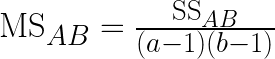
The first to calculate is the Sum of Square of factor A and B, which is just a column/row-wise squared sum of differences between the overall mean and column/row average (showing just row-wise calculation below)


We also have squared sum of interaction (i.e. each cell), defined as below (squared sum of average of each cell minus row average minus column average plus overall mean)

Also the error sum of square

Lastly we have total sum of square, which is the sum of all of the above, or we can validate by calculating the below (very useful to check if we are implementing it correctly)

Then we have the mean square error for each of the above (except total)


Lastly we calculate the test statistic F0 for factor A, B and interaction AB, by dividing the respective mean squared value with the mean squared error (MSError)
Next we find the critical value for each of them through the use of f.ppf
from scipy.stats import f

def critical_find(alpha, dof):
    return {
        "row": f.ppf(q=1 - alpha, dfn=dof["row"], dfd=dof["error"]),
        "column": f.ppf(q=1 - alpha, dfn=dof["column"], dfd=dof["error"]),
        "interaction": f.ppf(q=1 - alpha, dfn=dof["interaction"], dfd=dof["error"]),
    }
Where the degree of freedom (dof) for A, B and interaction AB are defined as

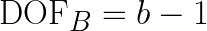

Putting together in a table, they become
 Source of Variation   |   Sum of Squares |   Degree of Freedom |   Mean Square |      F0 |       F | conclusion
-----------------------+------------------+---------------------+---------------+---------+---------+-------------------------
 factor a              |          3210.76 |                   4 |      802.689  | 73.8671 | 2.68963 | significant effect
 factor b              |          1193.73 |                   2 |      596.867  | 73.8671 | 3.31583 | significant effect
 interaction           |          5296.71 |                   8 |      662.089  | 60.9284 | 2.26616 | significant interaction
 Error                 |           326    |                  30 |       10.8667 |         |         |
 Total                 |         10027.2  |                  44 |               |         |         |
For factor A and B, we test to see if the effect is contributing to the sales by comparing the F0 with critical region, where the test hypothesis being
H0: has no effect to salesH1: has effect to sales
So for the case above, both factor A and B‘s F0 is greater than the critical value (the example uses alpha of 5%), so H0 is rejected and both factor significantly affect sales individually.
On the other hand, we also check if the interaction is significant. The hypothesis for this test is defined below
H0: no interaction between two factorsH1: there exists interaction between two factors
In this randomly generated example, as the F0 is also greater than the critical value, hence we reject the hypothesis. Therefore, if we want to further study if sales is affected, these two factors needs to be considered together.
Performing range test analysis
Range test analysis is then performed when interaction is significant. By fixing one of the factor, we are interested in finding out for each value of another factor, which contribute maximum or minimum sales (also finding which ones are having the same mean)
My old notes suggests the use of Duncan’s multiple range test, however in my previous implementation I used turkeyhsd provided by the statsmodel package. Considering I don’t know much about the test, I am skipping it here, however the interpretation of end result should be similar to Duncan’s multiple range test.
Performing Statistical Analysis with Panda DataFrame and SciPy
As I get more comfortable doing statistics with real world, I skipped implementing the formulas myself, finding it would be more efficient that way. The questionnaire itself is quite lengthy, and I was still inexperienced, so I only picked 12 variables to see if they are dependent on a set of social factors (age, gender etc.).
The social audit was to find out the reach of Internet access and technology to a community, which is a rather interesting project especially during this pandemic. Besides helping to setting up machines for their community library, I was also tasked to contribute to the final report with some statistical analysis to the survey data.
Test for independence
After picking a set of social factors X, and a set of variables Y, we proceed to form pairs from these two groups to test if they are associated. Chi-square test was picked for this purpose.
Then for those factors in X where we could somehow rank the responses (usually quantitative things like age, and certain categorical data that are in a sequence like colour order of rainbow, education level etc.), a test for correlation is done as well as the test for correlation significance.
First we would need to build a contingency table, where each row represents classes of X, and each column represent classes of Y. Each cell in the table represents the count of observation given the respective class of X and Y.
There are two types of X we find throughout the survey, i.e. either the values can be grouped into bins (continuous/discrete numbers e.g. age, or shopping budget) or the values are discrete (e.g. favourite colours).
On the other hand, based on the data we collected, we have three types of Y, i.e. the values that can be grouped into bins, distinct values, as well as questions where respondent can choose multiple options (require slightly different handling in code).
Therefore, in the end there are 6 different ways to create a contingency table. Which I would slowly go through some of them (the code can be found in the repository)
I am aware of the fact that the method I used might not be the most efficient, but my primary concern was to get it done correctly first. The library likely provides more efficient ways to achieve my goals. Also, the produced code really needs refactoring, I know that.
For instance, if we want to perform independence study on the education level of respondents and if they spend enough time on the Internet. These are both variables with distinct values (in a pandas.Series), hence we just put them side-by-side and start counting occurrences/observations:
import pandas as pd
from IPython.display import HTML, display

def distinct_vs_distinct(a, b, a_ranked):
    _df = pd.merge(
        a,
        b,
        left_index=True,
        right_index=True,
    )

    data = []

    for a_value in a_ranked:
        row = []
        for b_value in b.unique():
            _dfavalue = _df[_df[a.name] == a_value]
            row.append(_dfavalue[_dfavalue[b.name] == b_value].shape[0])

        data.append(row)

    result = pd.DataFrame(
        data,
        index=a_ranked,
        columns=pd.Series(b.unique(), name=b.name),
    )
    display(HTML(result.to_html()))
    result.plot(kind="line")

    return result_filter_zeros(result)


def result_filter_zeros(result):
    return result.loc[:, (result != 0).any(axis=0)][(result.T != 0).any()]


# First rank the education level
ranked_edulevel = pd.Series(
    [
        "Sekolah rendah",
        "Sekolah menengah",
        "Institusi pengajian tinggi",
    ],
    name=fields.FIELD_EDUCATION_LEVEL,
)

# Calling the function
edulevel_vs_sufficient_usage = relation.distinct_vs_distinct(
    normalized_edulevel, normalized_sufficient_usage, ranked_edulevel
)
It is always nice to have some sort of graphical reference, considering the code was running in a Jupyter Notebook so it is just too convenient to include the plot within the code. Considering X needs to be always ranked, hence the third parameter.
For variables where we group the responses into bins (e.g. household income, how much to pay monthly for internet access), the code varies slightly.
def interval_vs_interval(a, b, a_interval_list, b_interval_list):
    _df = pd.merge(
        a,
        b,
        left_index=True,
        right_index=True,
    )

    data = []

    for a_interval in a_interval_list:
        row = []
        for b_interval in b_interval_list:
            _dfamax = _df[_df[a.name] <= a_interval.right]
            _dfamin = _dfamax[a_interval.left < _dfamax[a.name]]
            _dfbmax = _dfamin[_dfamin[b.name] <= b_interval.right]
            row.append(_dfbmax[b_interval.left < _dfbmax[b.name]].shape[0])

        data.append(row)

    result = pd.DataFrame(data, index=a_interval_list, columns=b_interval_list)
    display(HTML(result.to_html()))
    result.plot(kind="line")

    return result_filter_zeros(result)


# Example calling
age_vs_budget_internet = relation.interval_vs_interval(
    normalized_age,
    normalized_budget_internet,
    summary_age.index,
    summary_budget_internet.index,
)
Overall, still not too difficult, as we are still only dealing with 2 series, it is still just counting the combination of pairs of values, which is somewhat similar to the previous case. It is just that now that both were intervals it takes more steps.
Next we have an example where we handle multiple choice questions (e.g. favourite websites). This is an example where the X values are binned, and Y is a multiple choice questions.
def interval_vs_mcq(a, b, a_interval_list):
    _df = pd.merge(
        a,
        b,
        left_index=True,
        right_index=True,
    )

    data = []

    for interval in a_interval_list:
        row = []
        for column in b.columns:
            _dfmax = _df[_df[a.name] <= interval.right]
            _dfmin = _dfmax[interval.left < _dfmax[a.name]]
            row.append(_dfmin[_dfmin[column] == True].shape[0])

        data.append(row)

    result = pd.DataFrame(data, index=a_interval_list, columns=b.columns)
    display(HTML(result.to_html()))
    result.plot(kind="line")

    return result_filter_zeros(result)
Though this time Y is a dataframe, but we are only finding out occurrences where a given pair of cases is true, so the code is more or less the same. The end product is still a contingency table that is ready to be processed later.
Then we are going to perform a test to find if Y is dependent on X, or they are both independent. So we first specify the null and alternative hypothesis.
H0: The two variables are independent (no relation)H1: The two variables are not independent (associated)
The alpha (error rate) is defaulted 0.05, which means should we repeat the survey, 95% of the time we would draw the same conclusion.
from scipy.stats import chi2, chi2_contingency

def independence_check(data, alpha=0.05):
test_stats, _, dof, _ = chi2_contingency(data)

critical = chi2.ppf(1 - alpha, dof)

independence = not independence_reject_hypothesis(test_stats, critical)

if independence:
print(
f"Failed to reject H_0 at alpha={alpha} since test statistic chi2={abs(test_stats)} < {critical}"
        )
    else:
        print(
            f"H_0 is rejected at alpha={alpha} since test statistic chi2={abs(test_stats)} >= {critical}"
)

return independence

def independence_reject_hypothesis(test_stats, critical):
return abs(test_stats) >= critical
As seen in the function, we just needed to pass in the contingency table we obtained previously into the chi2_contingency function then we quickly get test-statistic and the degree of freedom (we are ignoring the p-value here as we are going to calculate the critical region next). The test statistic can be calculated by hand with
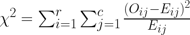
where
Oij= number of observations for the given classes in bothXandYEij= Expected value for each combination whenXandYare independent, which is just

Instead of flipping the distributions tables for the critical value, we can use chi2.ppf by passing in the confidence level (1 - alpha) and degree of freedom into it to find the critical value.
If the test statistic is greater than the critical value, i.e. falls outside the critical region, we reject the null hypothesis and conclude that both X and Y are associated. Otherwise, both variables are independent (a change in X does not affect Y), and we are not going to proceed any further.
Test for correlation
Now that we know both variables are associated, we shall perform a test for correlation next. Due to the data that we collected, they are either binned (e.g. age) or distinct ranked non-numeric data, so we are using Spearman’s Rank Correlation Coefficient,

where
rs= rank coefficient of correlationd= difference between two related ranksrX= rank of XrY= rank of Yn= number of pairs of observation

This time, as we know overall the changes in X affects Y, now we are interested in seeing how changes in X affects each value of Y. Besides finding out how they correlate, we are also interested in finding if the correlation is significant. If the correlation is significant, then the observation in our sample (the survey respondents) is also expected to be true in the population (all the residents in the community).
For this we conduct a two-tail test with the following hypothesis
H0: There is no significant correlation betweenXandYH1: There is a significant correlation betweenXandY
We are performing a t-test here as none of our data has more than 30 different pairs of observations of X and Y. Therefore the test statistic is
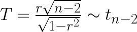
Again, welcome to the 21st century where nobody is flipping the distribution table for answer, t.ppf is used to calculate the critical value here.
from scipy.stats import t

def correlation_check(data, alpha=0.05, method="pearson"):
    _corr = (
        data.corrwith(
            pd.Series(
                range(len(data.index)) if method == "spearman" else data.index,
                index=data.index,
            ),
            method=method,
        )
        .rename("Correlation")
        .dropna()
    )
    display(HTML(_corr.to_frame().to_html()))

    critical = t.ppf(1 - alpha / 2, (len(_corr) - 2))

    for idx, rs in _corr.items():
        test_stats = rs * np.sqrt((len(_corr) - 2) / ((rs + 1.0) * (1.0 - rs)))

        print(
            f"The {(rs < 0) and 'negative ' or ''}correlation is {correlation_get_name(rs)} at rs={rs}."
        )

        if not correlation_reject_hypothesis(test_stats, critical):
            print(
                f"Failed to reject H_0 at alpha={alpha} since test statistic T={test_stats} and critical region=±{critical}. "
            )
            print(
                f"Hence, for {data.columns.name} at {idx}, the correlation IS NOT significant."
            )
        else:
            print(
                f"H_0 is rejected at alpha={alpha} since test statistic T={test_stats}, and critical region=±{critical}. "
            )
            print(
                f"Hence, for {data.columns.name} at {idx}, the correlation IS significant."
            )

        print()


def correlation_get_name(rs):
    result = None

    if abs(rs) == 1:
        result = "perfect"
    elif 0.8 <= abs(rs) < 1:
        result = "very high"
    elif 0.6 <= abs(rs) < 0.8:
        result = "high"
    elif 0.4 <= abs(rs) < 0.6:
        result = "some"
    elif 0.2 <= abs(rs) < 0.4:
        result = "low"
    elif 0.0 < abs(rs) < 0.2:
        result = "very low"
    elif abs(rs) == 0:
        result = "absent"
    else:
        raise Exception(f"Invalid rank at {rs}")

    return result


def correlation_reject_hypothesis(test_stats, critical):
    return abs(test_stats) > critical
Notice the value of data variable is just the same contingency table we generated in the previous step. This time we are interested in finding out the correlation of each class of Y compared to X, hence the loop in the code.
So by calling this function, we first get if there is a correlation between the class of Y, and then we further check to see if the correlation is significant.
Why is my current use of Jupyter notebook is not favourable
The whole report, if printed in A4 paper, is roughly 93 pages long. It is fine to have a glance of responses in the beginning during the cleaning/normalization part, however, towards the end where analysis starts, the nightmare begins.
Scrolling through a long notebook is not really fun. I am using the Visual Studio Code insider edition for the new Jupyter Notebook features, which makes it slightly easier to navigate because I could fold the notebook, which makes it slightly easier to find things. Should the questionnaire was longer, or if I were to do more analysis, referencing earlier parts of the notebook would be a nightmare.
Also, there are simply too many repeated code within the notebook. A lot of cells were there just to display the same contingency table and graph. It would be nice if I could reduce the repetition somehow.
Not sure if this can be properly fixed with Jupyter notebook, but I really wish I can break the notebook into multiple parts, and to be cross-referenced. Also, some sort of “metaprogramming” would be nice, so I stop having to repeat similar code in multiple cells.
Ending notes
I’m not too sure what comes in year 2021, but throughout 2020, being given an opportunity to work with a real Data scientist, and working on statistics analysis with real world data were great experiences. While I am not even close to be a real Data Scientist or even a Data Engineer, I am more interested in explore in these areas than ever.